Let’s read the document "sklearn.tree.DecisionTreeClassifier"

scikit-learn.org

• Click the [https://github.com/scikit-learn/scikit-learn/blob/42aff4e2e/sklearn/tree/_classes.py#L607:title=\[source\]] and check that the information in the website is provided in the source. ソースコードを見てみよう
  • The source file contains "python commands" and the information to be provided in the website and with help() function.
  • ソースファイルには、いわゆるパイソンのコマンドがあり、それ以外に、ウェブサイトに現れたりhelp()関数で呼び出したりする情報が書かれていることが解る
• What to know about 知っておくとよいこと
  • "Parameters" パラメタ(引数)
    • Parameters determine the conditions of "learning procedure" of the object you make.
    • パラメタは学習をするために作成したオブジェクトに、学習をするときの条件を与える
  • "Attributes" 属性
    • The python object to perform "learning" should have various information it needs to run and it generates during the run and information you want to know or to take out.
    • 属性は、学習を実行する際に必要な情報や、学習をさせた後で保持しておくべき、情報としてオブジェクトに付属してストックされる。属性は呼び出せる
  • "Methods" メソッド・関数
    • Methods are functions you can use with the object.
    • 学習用に作成したオブジェクトから使える関数のこと
    • The functions to perform the "learning" procedure itself are included.
    • 学習を実施するには、入力を取っていろいろなことをしないいけないが、そのするべきことが関数として指定されている。その関数が含まれる
    • Also the functions useful to process the inputs and outputs so that the users feel comfortable to use the object.
    • その他に、学習の入出をいじったり加工したりできると便利なので、便利関数がオブジェクトから呼び出せるようになっている
• Python commands
  • Show parameters and attributes (splitter is a parameter. max_features_ is an attribute)
  • パラメタと属性を表示させてみる

clf.splitter

clf.max_features_

• • Another way to get the value of parameters/attributes

getattr(clf,"max_features_")
getattr(clf,"splitter")

• • Use a function in Methods. メソッド登録されている関数を使ってみる
    • Learn and generate a model

clf.fit(X,y)

• • • Use the generated model

clf.predict(X)

• ipynb

github.com

Decision Tree & Graphviz、pip, conda を使う

• Visit this site for the original codes.
• Start your jupyter notebook　ジュピターノートブックを開始する
  • (1) Start your "Anaconda navigator" then select jupyter notebook. アナコンダ・ナビゲータを立ち上げて、そのメニューからジュピターノートブックを立ち上げてもよい
  • (2) Or start "jupyter notebook" directly. You can type "jupyter notebook" in your terminal for this. ジュピターノートブックを直接立ち上げてもよい。ターミナルに"jupyter notebook"と打ち込んで立ち上げることもできる
• Open a new jupyter notebook with "python3" kernel in your browser. 新しいジュピターノートブック(カーネルはpython3)をブラウザで開く
• Write (or copy-and-paste) the following python commands 以下のパイソンコマンドをノートブックに書きます(コピーペーストします)
  • Each section should be filled in each chunk. 一区切りごとに１チャンクに書き込みます
• We will encounter various errors, but let's solve them one by one. エラーが続出すると思いますが、一つずつ解決していきます

# The following codes are borrowed from https://qiita.com/Hawaii/items/53efe3e96b1171ebc7db 
# pandas for Data structure "dataframe"
# numpy for matrix-like data structure
# sklearn for machine learning
import pandas as pd
import numpy as np
from sklearn.tree import DecisionTreeClassifier, export_graphviz

# To make an image of "decision-tree" and display
# Non-python application "Graphviz" is required
# this python package "graphviz" connects NON-python application "Graphviz" into python environment
import graphviz 
# python package to assist Graphviz functionality
import pydotplus 
# something to show the image in jupyter notebook 
from IPython.display import Image 
# something to show the image in jupyter notebook (environment dependency is likely) 
from sklearn.externals.six import StringIO 
# If you get an error from the above line, try
# from io import StringIO 

data = pd.DataFrame({
        "buy(y)":[True,True,True,True,True,True,True,False,False,False,False,False,False],
        "high":[4, 5, 3, 1, 6, 3, 4, 1, 2, 1, 1,1,3],
        "size":[30, 45, 32, 20, 35, 40, 38, 20, 18, 20, 22,24,25],
        "autolock":[1, 0, 1, 1, 1, 1, 1, 0, 0, 0, 0,1,0]
    })

y = data.loc[:,["buy(y)"]]
X = data.loc[:,["high", "size","autolock"]]

clf = DecisionTreeClassifier()
clf = clf.fit(X, y)

# Mac
dot_data = StringIO() # "dot-format" information for "tree-graph" will be stocked
export_graphviz(clf, out_file=dot_data,  
                     feature_names=["high", "size","autolock"], 
                     class_names=["False","True"],  
                     filled=True, rounded=True,  
                     special_characters=True) 
graph = pydotplus.graph_from_dot_data(dot_data.getvalue())
#graph.progs = {'dot': u"C:\\tools\\Anaconda3\\Library\\bin\\dot.bat"}  # 追加部分

Image(graph.create_png())

# Windows
dot_data = StringIO() # "dot-format" information for "tree-graph" will be stocked
export_graphviz(clf, out_file=dot_data,  
                     feature_names=["high", "size","autolock"], 
                     class_names=["False","True"],  
                     filled=True, rounded=True,  
                     special_characters=True) 
graph = pydotplus.graph_from_dot_data(dot_data.getvalue())
graph.progs = {'dot': u"C:\\tools\\Anaconda3\\Library\\bin\\dot.bat"}  # Windows
#C:\tools\Anaconda3\Library\bin\dot.bat
# graph.progs = {'dot': u"C:\\Users\\ryamada\\Anaconda3\\Library\\bin\\dot.bat"} 
# worked in another Windows environment.
Image(graph.create_png())

print(graph.to_string())

• pip
  • Open the regular terminal

pip install --upgrade pip

• • Install the packages if you get errors @ import xxxx

pip install xxxx

• conda
  • Graphviz is a graph visualization application. Graphviz はパイソンから独立したグラフ描図アプリ

graphviz.org

• • Graphviz can be installed in your local PC, either Mac or Windows... ダウンロードしてMac/WindowsのローカルPC上でも使えます
  • In my environment, python3 on jupyter notebook was able to call the installed Graphviz without further settings.
  • In my environment, python3 on jupyter notebook failed to call the installed Graphviz (probably "path-problem"). Therefore, a python code line was added to specify the location of installed Graphviz's "dot"-functionality command file "dot.bat", based on an instruction here

niwakomablog.com.

• • • The "dot.bat", that was called from python to generate an image by Graphviz, was created by the command "conda install graphviz" . Windowsの場合、"dot.bat"というファイルをpython内から呼び出して、Graphvizに図を作らせていますが、それは"conda install graphviz"というコマンドで作られたものです

conda install graphviz

• • • It installed "Graphviz" under the Anaconda folder in my windows PC: "C:\\tools\\Anaconda3\\Library\\bin\\dot.bat" WindowsではそのコマンドによりAnaconda関連の一式を納めた領域にGraphvizがインストールされます。
    • As far as searched the websites, various errors/troubles around Graphviz and python connection. Graphvizをpythonで使うためにはいろいろな方法でGraphvizをインストールすることができるようです(難航した人が結構、存在する、ということの裏返し)
• If no solution, print out "dot-formatted string" and copy-and-paste the contents to the Graphviz-online. もしpythonからのGraphviz呼び出しに成功しなかったり、そもそもGraphvizがローカルPCで動かない場合には、pythonでGraphvizが受け付ける「グラフを描くための文字列」を作って、それを「Graphvizをウェブサイト上で動かすサイト」に持っていくという手もあります

dreampuf.github.io

print(graph.to_string())

digraph Tree {
node [color="black", fontname=helvetica, shape=box, style="filled, rounded"];
edge [fontname=helvetica];
0 [fillcolor="#399de524", label=<size &le; 27.5<br/>gini = 0.497<br/>samples = 13<br/>value = [6, 7]<br/>class = True>];
1 [fillcolor="#e58139d4", label=<autolock &le; 0.5<br/>gini = 0.245<br/>samples = 7<br/>value = [6, 1]<br/>class = False>];
0 -> 1  [headlabel="True", labelangle=45, labeldistance="2.5"];
2 [fillcolor="#e58139ff", label=<gini = 0.0<br/>samples = 5<br/>value = [5, 0]<br/>class = False>];
1 -> 2;
3 [fillcolor="#e5813900", label=<size &le; 22.0<br/>gini = 0.5<br/>samples = 2<br/>value = [1, 1]<br/>class = False>];
1 -> 3;
4 [fillcolor="#399de5ff", label=<gini = 0.0<br/>samples = 1<br/>value = [0, 1]<br/>class = True>];
3 -> 4;
5 [fillcolor="#e58139ff", label=<gini = 0.0<br/>samples = 1<br/>value = [1, 0]<br/>class = False>];
3 -> 5;
6 [fillcolor="#399de5ff", label=<gini = 0.0<br/>samples = 6<br/>value = [0, 6]<br/>class = True>];
0 -> 6  [headlabel="False", labelangle="-45", labeldistance="2.5"];
}

• Regular terminal & Anaconda terminal
• You can get the jupyter notebook file here: 以上のpythonコマンドをjupyter notebook形式で保存したものは、以下から取れます

github.com

Add library/package ライブラリ/パッケージの追加 pip, conda

• Library > Package > Module
  • Different terms... but, simply speaking, something you can get and use for your study.
  • 名前が色々あるけれど、簡単に言えば、「取ってきて使うもの」
• PyPI : Py-thon P-ackage I-ndex

pypi.org

• • python's libraries and packages are registered.
  • パイソンのライブラリ/パッケージが登録してある
  • Use pip command to install libraries/packages you want to use from the registry.
  • pip コマンドを使って、使いたいライブラリ/パッケージを取って来る
    • The command "pip" itself should be updated so that you can get the latest libraries/packages.
    • コマンド "pip"自体を最新にして、最新のレジストリからライブラリ/パッケージを取って来る

pip install --upgrade pip

pip install hoge

• "conda"
  • The command "conda" is to get something you use in your Anaconda-based environment.
  • "conda"コマンドはアナコンダを使った作業環境に使用したいものを取って来るコマンド
  • It gets python libraries/packages as well as other tools.
  • pythonのライブラリ/パッケージも取って来るが、それ以外のツールも取って来る
  • It brings them into your Anaconda-environment.
  • 取ってきたものは、アナコンダが管理した環境で使えるようになる
  • The command pip and the command conda can be used together.... This makes the beginners confused further.
  • pip コマンドとconda コマンドとは併用もできるので、さらに混乱しますが…
    • The famous libraries/packages are well maintained by both pip-system and conda-system and you might not find big trouble by the choice of pip vs. conda.
    • 有名どころのライブラリ/パッケージはよくメンテナンスされているので、pipを使うかcondaを使うかで問題に巻き込まれることは少ないかもしれません。

www.anaconda.com

• Environment to use python パイソンの使用環境
  • You can make your computer do your tasks with python commands. The tasks are achieved with the communicating network of "python" itself and python's libraries/packages you downloaded with or without non-python applications.
  • パイソンのコマンドを発行することで、コンピュータに仕事をやらせているとき、"python"の本体と、ダウンロードしてきたパイソンのライブラリ/パッケージと、場合によってはパイソンに属さないアプリとを連携したネットワークを使っている
  • Python you installed without Anaconda, python already installed when you bought your PC, python you installed with Anaconda..., they behave differently.
  • Anacondaを使わずにインストールしたパイソンと、PCを買ったときにすでに入っているパイソンと、アナコンダを使ってインストールしたパイソン.... これらの挙動は違います
  • To control these differences, you should pay attention to the different terminals you can use.
  • これらの違いをコントロールするために、使える「ターミナル」の違いに注意する必要があります
    • The regular terminal of your PC. PCのターミナル
    • The terminal you access as a part of Anaconda. アナコンダの一部になっているターミナル
  • It is not wise to learn all the backgrounds of this topic before enjoy the data analysis, but this knowledge will give you hints for the troubles you will face in future. I hope your net-surfing skills to solve the troubles become adequate before you face the first trouble of this kind.
  • ここで言うトピックの背景について勉強を終えてからデータサイエンスをするのは得策ではないですが、このことを少しでも聞いておくと、いざ、トラブルに見舞われたときのとっかかりになるので書いておきます。いざ、この手のトラブルに見舞われたとき、コンピュータスキルが上がっていて、自力でネットサーフするなどして問題解決できるようになっていることを祈ります

Install Anaconda, Anacondaのインストール

• Let's use Anaconda。Anacondaを使う

www.anaconda.com

• • Why? どうして？ (1)
    • It provides basic libraries/packages for data science (numpy, scipy, pandas).
    • データサイエンス用の基本ライブラリ・パッケージが入っているから (numpy, scipy, pandas)
    • numpy: matrix, linear algebra 行列と線形代数
    • scipy: mathematical functions 数学の関数
    • pandas: data stocking structures and analysis functions for statistical analysis 統計解析用のデータ格納構造と解析関数
  • Why? どうして? (2)
    • It provides Jupyter-notebook, useful to make your skills better and to record your activities.
    • Jupyter-notebookという、スキルアップと記録保存に便利なツールがついているから
• How to install Anaconda in English
  • Mac

docs.anaconda.com

• • Win

docs.anaconda.com

• アナコンダのインストール方法(日本語)
  • Mac

www.python.jp

• • Win

www.python.jp

numpy.ndarray と Rのapply()

• Rの行列で、各行の和を出そうと思ったら

M <- matrix(rnorm(100),10,10)
apply(M,1,sum)

• だろう
• 同じことをPythonでやるのはどうするのかな、と思った
• Pythonで行列を扱うならnumpyがよいのでそうすることにしたとして
• 値のセットの和を出すsum()関数を、軸方向に指定して計算することもできて

M = np.array(np.random.randint(5,18000,100)).reshape(10,10)
np.sum(M,axis=1)

• とするらしい。Rのapply(M,1,sum)と同じ構成
• それとは別に：
• numpyのndarrayにはuniversal functionsというのがある。名前は「大層」だが、全要素に同じ処理をして、同じサイズのndarrayを作る関数のこと(種類がたくさんある)
• このuniversal functionを繰り返し使って、答えをたたんでいくという処理をしろ、という指示である、reduceという「高階関数」と組み合わせるらしい

M = np.array(np.random.randint(5,18000,100)).reshape(10,10)
np.add.reduce(M,axis=1)

• ちなみに、universal functionsのリストはここにある
• また、recude以外にも、「高階関数的ndarray処理」として、以下のようなものがあるらしい。どういううまみがあるのかまだわからない
  • ufunc.reduce(a[, axis, dtype, out, …])
    • Reduces a’s dimension by one, by applying ufunc along one axis.
  • ufunc.accumulate(array[, axis, dtype, out])
    • Accumulate the result of applying the operator to all elements.
  • ufunc.reduceat(a, indices[, axis, dtype, out])
    • Performs a (local) reduce with specified slices over a single axis.
  • ufunc.outer(A, B, **kwargs)
    • Apply the ufunc op to all pairs (a, b) with a in A and b in B.
  • ufunc.at(a, indices[, b])
    • Performs unbuffered in place operation on operand ‘a’ for elements specified by ‘indices’.
• reduceのほかに、基本となる「高階関数」についてはこちらなどで。

RとPythonの両方で使えるplotlyでの3Dスキャタープロットを覚える

• Rもpythonもjupyter notebookで文書作成できる
• ３次元プロットをしなくてよいのなら、Rでは普通の二次元プロッティング関数を使えばよいし、Pythonではmatplotlibを使えばよい
• ３次元プロットを描いてぐりぐり動かすとなると、Rではplot3dを使い、pythonでは…、plotlyが使えるか…となる
• が、両方を別々に覚えるのが、記憶力の減退と共につらい
• jupyter notebook上ならＲもPythonもplotlyで3Dぐりぐりができるということらしいので、両者を比較しながら、使ってみることにする
• 準備
  • R

install.packages("plotly")

• • として

library(plotly)

• • で、準備OK
  • Python

pip install plotly

• • が必要なのは陶然として、jupyter内で動かすには

pip install npm
jupyter labextension install @jupyterlab/plotly-extension

• • としないと、plotlyの画像出力がjupyter notebook上に現れない

import plotly.offline as offline
import plotly.graph_objs as go
offline.init_notebook_mode()

• • として、ようやく、offline.iplot()関数にpyplotで作ったグラフ表示情報オブジェクトを渡すことで、グラフが現れる
• 散布図
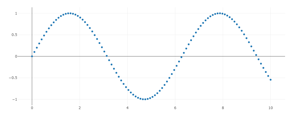
  • Rの場合

p <- seq(from=0,to=1,length=100) * 10
q <- sin(p)
fig = plot_ly(x=p,y=q,type="scatter")
fig

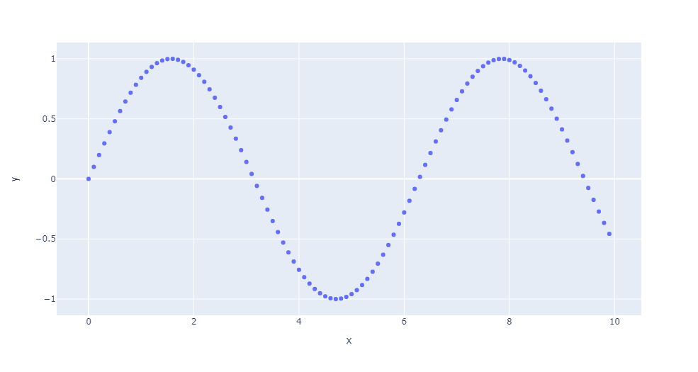
• • Pythonの場合
  • もともとのplotlyはplotly.graph_objsという仕様で、細かく描画条件を指定するようになっているらしいが、さすがに面倒だ、ということで、簡単にした(機能を落としつつ、コマンドを簡略化した)plotly.expressというものがある。以下ではそれを使う

import numpy
import plotly.express as px
p = numpy.arange(100) * 0.1
q = numpy.sin(p)
fig = px.scatter(x=p, y=q)
fig.show()

• • ちなみにこのplotly.expressはplotly.graph_objects.Figureを返すので、fig.show()　として描画することも、offline.iplot()として描画することもできるようである
• 3D scatter plot
  • Rの場合(このブログでは動かせないがjupyter notebook上では動かせる)

xyz <- matrix(rnorm(10000*3),ncol=3)
xyz <- xyz/sqrt(apply(xyz^2,1,sum))
fig2 <- plot_ly(x=xyz[,1],y=xyz[,2],z=xyz[,3],type="scatter3d",marker=list(size=1,color=xyz[,3]))
fig2

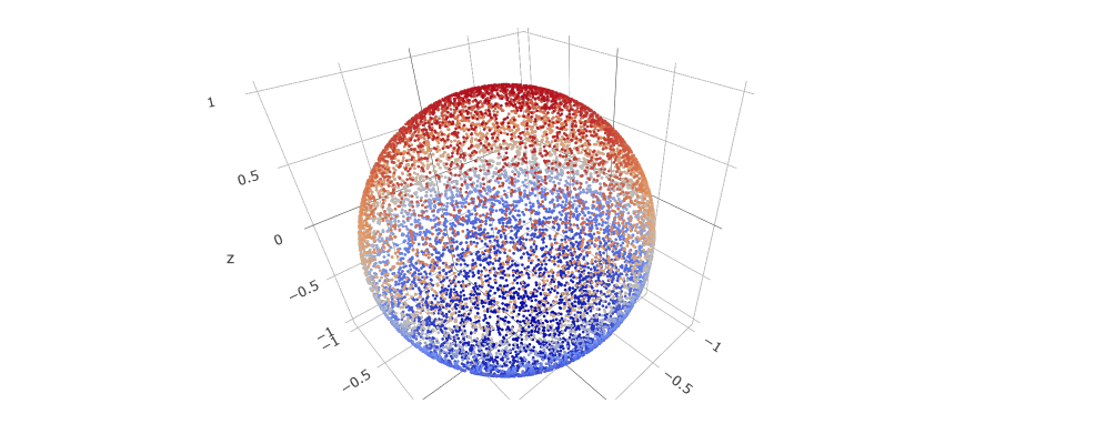
• • Pythonの場合
    • 2D scatterplotではplotly.expressを使ったが、3D scatterplotだと、点のサイズ指定で(少なくとも自分の環境では)エラーがでるので、簡易版expressではなく、plotly.graph_objsを使うこととする

import plotly.offline as offline
import plotly.graph_objs as go
offline.init_notebook_mode()

import numpy 
import numpy.random
def my_unit_vector(X):
    return(X/numpy.linalg.norm(X,axis=1).reshape(-1,1))
    
xyz = numpy.array(numpy.random.randn(1000,3))
xyz_ = my_unit_vector(xyz)

trace = go.Scatter3d(
   x = xyz_[:,0], y = xyz_[:,1], z = xyz_[:,2],mode = 'markers', marker = dict(
      size = 1)
   )
fig = go.Figure(data = [trace])
offline.iplot(fig)

• • 以下のように、描くべきオブジェクト fig を作って、offline.plot()に渡すだけでも描ける

fig = go.Figure(go.Scatter3d(x = xyz_[:,0], y = xyz_[:,1], z = xyz_[:,2],mode = 'markers', marker = dict(size = 1)))
offline.iplot(fig)

• • 最後の描画のところは、offline.iplot(fig)の代わりに

fig.show()

• • でも３Dぐりぐりプロットが現れる(ようだ)
  • もう、細かいことはいいから、Rのplot3d()的に描ければいいや、ということなら、関数を定義して

def my_go_scatter3d(X,size=1):
    fig = go.Figure(go.Scatter3d(x =X[:,0], y = X[:,1], z = X[:,2],mode = 'markers', marker = dict(size = size)))
    offline.iplot(fig)

my_go_scatter3d(xyz_)

• • でもよいようだ
• pythonのnumpy.apply_along_axis()関数
  • 上述の単位球面乱数座標生成では、

def my_unit_vector(X):
    return(X/numpy.linalg.norm(X,axis=1).reshape(-1,1))

• • という関数を定義して使った。これは、numpyの線形代数関連関数を納めたlinalg配下にあるnormを取る関数を列(axis=1)に関してつぶした結果を返すという処理。この処理は(おそらく)高速実装されている。
  • これに似たやり方で、自作の関数 my_fun()を定義して、同様に、numpy ndarrayに作用するには

numpy.apply_along_axis(my_fun,axis=1,m) 

• • のようにして、ndarray オブジェクトm(行列と仮定しておく)の列(axis=1)をつぶすようにmy_fun()を各行に処理させることができる
  • ただし、これは、ループ処理を簡略化して書いてあるだけなので、mの各要素にアクセスするそうで、速くなるわけではないらしい(Rのapply()関数は、場合によっては、ベクトル演算化できるところはベクトル演算化して速くしてくれたはずだが…。要するに、Rで言えばlapply()関数的なものということなのだろう)
  • それよりは、ベクトル化した(必要ならループを使った)コードを書く方が速いらしい(参考はこちら)
• Python の plotlyは、pythonのディクショナリ形式で必要な情報を持たせて、それをplotly.graph_objects.Figure 形式に修正してFigureデータタイプで持たせ、その情報を読んで視覚化する、という仕組み：こちら。
• それが解れば、あとは、例(https://plotly.com/python/:tilte=こちら)を参考に、合わせて行けばよいようだ

ぱらぱらめくる『Nature Reviews Genetics』2020

• １細胞データに付加価値(採取場所情報、細胞間関係情報、細胞集合としての分布取得、など)を付ける話が目立つようです。
• 12月号
  • Genotype–Tissue Expression (GTEx) 最新の成果についてのコメント。GTExのポータルで検索可能
    • "The data set of 838 donors and 15,201 samples across 49 tissues"
    • "4,278,636 genetic variants were associated with gene expression. At least one associated cis expression quantitative trait locus (cis-eQTL) was identified for 94.7% of all protein-coding genes. "
  • Transposable elements (TEs)のNGS発現リードを捨てずに使う
  • エピゲノムと細胞代謝
    • "linking the environment to the maintenance of cellular homeostasis and cell identity"に関与する代謝物が広範に及ぶ由
• 11月号
  • クロマチンの3D構造解析。直接観察のスループットを上げる手法
  • データを集めやすく、かつ、複雑な表現型として、血球集合を選び、大規模遺伝因子探索
  • cell competition and super-competition were recognized in mammalian development, organ homeostasis and cancer
• 10月号
  • memory sequencing (MemorySeq), a method for identifying genes that are highly and heritably expressed over multiple cell divisions
  • Chromatin accessibility profiles and other omics data to prioritize neuropsychiatric-disease-associated genetic variants and to identify potential gene regulatory mechanisms underlying the pathology
  • 分化発生による発現パターンの違いを記述統計にとどめず、１細胞・介入で因果関係解明に持ちこむ
  • https://www.nature.com/articles/s41576-020-0272-6:genetics/genomicsの展望総説
• 9月号
  • A new study presents a spatial transcriptomics technique called ZipSeq, whereby patterned illumination is used to print barcodes onto chosen tissue regions １細胞トランスクリプトームしつつ、各細胞を取ってきた「空間情報」を失わずに取るための方法
  • 種による加齢速度の違いをエピゲノムで
  • 臓器組織別の再生可能性の違いの解明
• 8月号
  • 精子の１細胞シークエンシングによる減数分裂変異の解析
  • genetic variation for 15,708 whole genomes in addition to 125,748 exomes. The increase in sample size and inclusion of non-coding regions yielded more than 240 million small genetic variants as well as structural variation
    • gnomADのサイト
  • Electronic health records and polygenic risk scores for predicting disease risk
• 7月号
  • Lineage tracing meets single-cell omics: opportunities and challenges
  • Phylogenetic tree building in the genomic age
• 6月号
  • Higher-order chromatin structure undergoes dynamic change & chromatin dynamics and allele-specific gene expression during early mouse embryogenesis
• 5月号
  • Transcriptional profiling of physically interacting cells
• 4月号
  • Methods for mapping 3D chromosome architecture
  • ‘pan-genomes’, which are reference genomes that encompass the genetic variation within a given species
• 3月号
  • 放っておくとこういう風に進むという'default' way
  • 構造多型検出
• 2月号
  • Mosaic loss of chromosome Y (LOY)と癌や加齢性疾患との関係
  • Determinants of enhancer and promoter activities of regulatory elements
  • 加齢の遺伝学
• 1月号
  • A statistical framework for rare disease diagnosis